import matplotlib.pyplot as plt
import numpy as np
import pandas as pd
import plotly.graph_objects as go
from IPython.display import Markdown, display
from plotly.subplots import make_subplots
from scipy.optimize import curve_fit
Read in Data
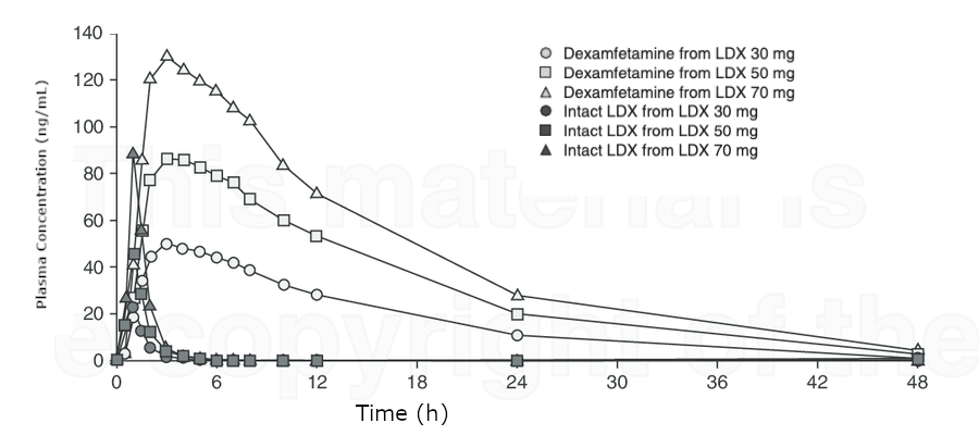
Let's read in data from Steer C, Froelich J, Soutullo CA, Johnson M, Shaw M . (). Lisdexamfetamine dimesylate: a new therapeutic option for attention-deficit hyperactivity disorder.
Well we are not reading it from there, I manually extracted them :-).
 Plasma concentration-time profile of lisdexamfetamine and lisdexamfetamine-derived dexamfetamine (reproduced from Boellner et al., [18], ª 2010). LDX = lisdexamfetamine dimesylate.
df = pd.read_csv("ldx_over_time.csv").dropna()
df
| time | 30mg | 50mg | 70mg | |
|---|---|---|---|---|
| 0 | 0.0 | 0.0 | 0.0 | 0.0 |
| 1 | 0.5 | 5.0 | 15.0 | 20.0 |
| 2 | 1.0 | 18.0 | 27.0 | 40.0 |
| 3 | 1.5 | 35.0 | 55.0 | 85.0 |
| 4 | 2.0 | 45.0 | 78.0 | 120.0 |
| 5 | 3.0 | 50.0 | 87.0 | 130.0 |
| 6 | 4.0 | 48.0 | 86.0 | 125.0 |
| 7 | 5.0 | 47.0 | 84.0 | 120.0 |
| 8 | 6.0 | 45.0 | 80.0 | 115.0 |
| 9 | 7.0 | 42.0 | 78.0 | 110.0 |
| 10 | 8.0 | 39.0 | 70.0 | 103.0 |
| 12 | 10.0 | 33.0 | 60.0 | 85.0 |
| 14 | 12.0 | 28.0 | 53.0 | 72.0 |
| 17 | 14.0 | 0.0 | 0.0 | 0.0 |
We will fit a bi-exponential model
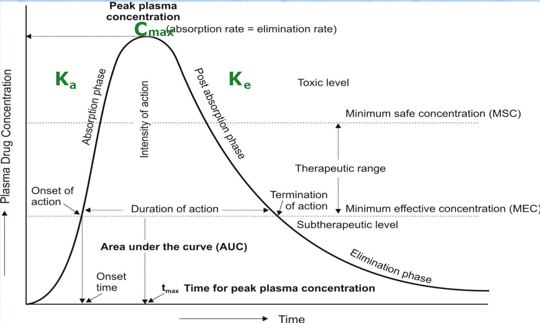
As we can see from the modeling of Pharmacokinetics, a bi-exponential model seems appropriate. See:Centurion University of Technology and Management. (2021). Pharmacokinetic Models. Retrieved from https://course.cutm.ac.in/wp-content/uploads/2021/03/pharmacokineticmodels.pdf

So in essence we are modelling $$ \left( \frac{C_{\text{max}} \cdot K_a}{K_a - K_e} \right) \left( e^{-K_e \cdot t} - e^{-K_a \cdot t} \right) $$
And we are fitting the parameters:
- $C_{\text{max}} = $ Peak Plasma Concentraion
- $K_a =$ Absorption Factor
- $K_e =$ Elimination Factor
# Define the bi-exponential model
def bi_exponential(t, Cmax, Ka, Ke):
    return (Cmax * Ka / (Ka - Ke)) * (np.exp(-Ke * t) - np.exp(-Ka * t))


# Prepare your data for fitting
times = np.tile(df["time"].values, 3)  # Repeat time values for each dose
# Stack concentration values for all doses, effectively treating them as one dataset
concentrations = np.hstack((df["30mg"].values, df["50mg"].values, df["70mg"].values))
# Stack the doses, repeated for the length of the time vector
doses = np.hstack(
    (
        np.full(df["time"].size, 30),
        np.full(df["time"].size, 50),
        np.full(df["time"].size, 70),
    )
)
# Initial parameter estimates (Cmax, Ka, Ke) - these are guesses and might need to be refined
initial_params = [concentrations.max(), 1, 0.1]


# Curve fitting with dose as a scaling factor
def fit_function(t, Cmax, Ka, Ke):
    return bi_exponential(t, Cmax, Ka, Ke) * doses[: len(t)]


params, covariance = curve_fit(fit_function, times, concentrations, p0=initial_params)
# Function to calculate model predictions using the fitted parameters
def predict_concentration(t, Cmax, Ka, Ke, dose):
    return bi_exponential(t, Cmax, Ka, Ke) * dose
# Generate predictions using the fitted parameters for each dose level
time_continuous = np.linspace(df["time"].min(), df["time"].max(), 100)
predictions_30mg = predict_concentration(time_continuous, *params, 30)
predictions_50mg = predict_concentration(time_continuous, *params, 50)
predictions_70mg = predict_concentration(time_continuous, *params, 70)
# Increase Ke for quicker decay
# quicker_Ke = params[2] * 2  # Example of making the decay faster
# New parameters with quicker decay
params = (params[0], params[1], 3 * params[2])
# Plot the original data and the fits
plt.figure(figsize=(12, 6))
# Original data
plt.scatter(df["time"], df["30mg"], label="Original 30mg", color="red", s=10)
plt.scatter(df["time"], df["50mg"], label="Original 50mg", color="green", s=10)
plt.scatter(df["time"], df["70mg"], label="Original 70mg", color="blue", s=10)
# Fitted curves
plt.plot(
    time_continuous, predictions_30mg, label="Fit 30mg", color="red", linestyle="dashed"
)
plt.plot(
    time_continuous,
    predictions_50mg,
    label="Fit 50mg",
    color="green",
    linestyle="dashed",
)
plt.plot(
    time_continuous,
    predictions_70mg,
    label="Fit 70mg",
    color="blue",
    linestyle="dashed",
)

plt.xlabel("Time (hours)")
plt.ylabel("Concentration (ng/mL)")
plt.title("Pharmacokinetic Model Fit to Multiple Doses")
plt.legend()
plt.grid(True)
plt.show()
markdown_template = """
# Results
This worked great. To give more practical feedback $K_e$ has been manually slightly adjusted. So that:
$$
\\left( \\frac{{C_{{\\text{{max}}}} \\cdot K_a}}{{K_a - K_e}} \\right) \\left( e^{{-K_e \\cdot t}} - e^{{-K_a \\cdot t}} \\right)
$$

With the fitted values:
- $C_{{\\text{{max}}}} =$ {params[0]}
- $K_a =$ {params[1]}
- $K_e =$ {params[2]}
"""

# Replace placeholders with the actual values
markdown_text = markdown_template.format(params=params)
# Cmax=params[0], Ka=params[1], Ke=params[2])

# Display the formatted markdown
display(Markdown(markdown_text))
Results
This worked great. To give more practical feedback $K_e$ has been manually slightly adjusted. So that: $$ \left( \frac{C_{\text{max}} \cdot K_a}{K_a - K_e} \right) \left( e^{-K_e \cdot t} - e^{-K_a \cdot t} \right) $$
With the fitted values:
- $C_{\text{max}} =$ 4.816931830999022
- $K_a =$ 0.23815199140828144
- $K_e =$ 0.7144975482181155
params
(4.816931830999022, 0.23815199140828144, 0.7144975482181155)